Time-series foundation models for building control?

At EnergyWise, we develop software to optimize heating, ventilation and air-conditioning in buildings. The objective is to reduce energy consumption while maintaining occupant comfort. In practice, this means making decisions about equipment: when to start it, which setpoint to use, or how to adapt its operation to changing conditions.

A recurring challenge is understanding how each building responds to those decisions. Spaces with similar temperatures can behave differently once heating starts, depending on their thermal mass, insulation, equipment and exposure. As we discussed in our article on scaling AI-driven HVAC control, the engineering effort needed to model each new environment is a substantial part of the deployment problem.

Time series foundation models are a new class of ML models, pretrained on large collections of time series, that can be applied to a wide range of time series tasks, including forecasting.

Theoretically, here, instead of training a new model for every zone, we would provide a window of historical measurements and ask it to predict what comes next. In a zero-shot setting, we’d do this without updating the model’s parameters for the target building.

Having a reusable model could help with temperature prediction, equipment scheduling, demand response or evaluating candidate control strategies. And also reduce the amount of building-specific modeling needed for an optimization service.

However, being a good forecaster doesn’t mean the model actually learns the underlying thermal dynamics.

We’ll explore the problem in this article, trying to answer the question:

Can a model that forecasts indoor temperature also predict what happens when we change the control?

We’ll explore this through a simple optimal-start experiment with Timestral and EnergyPlus, and connect the results to recent research.

From forecasting to counterfactual analysis

Consider optimal start problem: choosing when to start heating so that a room is comfortable when people arrive. The goal is to minimize energy use while ensuring the room reaches its setpoint at the right time.

An ordinary forecast answers: given the recent history and the usual schedule, when will the room reach its setpoint?

For optimization, we also need to ask: what if we start 30 minutes later? Or one hour earlier? This is counterfactual analysis: comparing what would happen under an alternative action with what happens under a reference action, under otherwise comparable conditions.

Our problem statement is therefore:

Given a zone’s recent temperature history, weather and operating schedules, can a pretrained model predict how shifting the HVAC start changes the time at which comfort is reached?

To answer this well, the model needs to capture the causal effect of the action. It must distinguish the temperature change caused by HVAC operation from changes associated with weather, solar gains or the daily routine.

Learning that distinction can be difficult. If heating always starts at the same time, its activation, the setpoint change and the morning temperature rise tend to occur together. A model can learn that pattern and forecast it accurately. When we separate those events by changing the schedule, we discover whether it has also learned how the system responds to the command.

Here the target is indoor temperature. Outdoor temperature, the heating setpoint and the HVAC availability command are covariates.

Some covariates are available only in the past, such as measured heating power. Others can be supplied over the forecast horizon: a weather forecast, a planned setpoint, or a candidate on/off schedule. These are commonly called known-future covariates, although a future weather value may itself be a forecast.

Timestral is capable of using both types of covariates, which is important for our experiment. This gives us a convenient way to query a model: supply several candidate HVAC schedules and compare the resulting temperature predictions.

What does recent research tell us?

Three recent papers approach this question from complementary directions:

Study	Main idea and connection to our experiment
Amria et al., Time-series Foundation Models for Predictive Control: The Role of Excitation, 2026 preprint	In residential heat-pump experiments, the authors distinguish ordinary forecasting accuracy from accuracy under changed control inputs. Their Chronos-2 results show that sufficient independent control variation in the context can help recover the input-response relationship. This suggests that the information contained in the history matters as much as the ability to accept future controls.
Wang, ThermoForce, 2026 preprint	This work keeps a foundation model frozen to predict the passive component of temperature evolution, and learns a small physics-structured operator for the HVAC response. Its paired EnergyPlus experiments explicitly evaluate intervention effects. A good forecast under existing operation does not validate predictions under different actions.
Liang et al., ThermoStill, ACM e-Energy 2026	ThermoStill transfers knowledge from multiple TSFMs into a physically consistent resistance-capacitance (RC) model, which represents heat transfer and storage. The authors evaluate the approach in BOPTEST and a real meeting room. This illustrates another role for foundation models: helping train a compact thermal model that a controller can use.

These studies give us reasons to investigate further. They explore required predictor context, model adaptation and physical structures, that can turn a good forecast into a good counterfactual predictor.

Our experiment asks a narrower, practical question: what happens if we take a model with native covariate support and use it directly, zero-shot, for a zone-level scheduling decision?

A simple experiment: move the start time

We use Timestral-209M, without fine-tuning, to forecast one simulated zone across 30 mornings. Each forecast receives ten days of history, with measurements every 15 minutes. Future inputs include HVAC availability, heating setpoint and outdoor temperature; weather is supplied from the simulation.

EnergyPlus provides the reference trajectories. We run the building model with its baseline schedule, then re-run it with earlier or later HVAC starts. This lets us observe the simulated outcome of the actions we want to compare.

We separate the experiment into two questions:

Test	Question
T1: observed accuracy	With the baseline schedule unchanged, can Timestral predict when the zone reaches its heating target?
T2: counterfactual accuracy	On the same dates, if we shift the start by −60, −30, +30 or +60 minutes, does it predict the resulting change in comfort time?

For T2, all candidate schedules are forecast from the same issue time, before the earliest start. We change HVAC availability while keeping the setpoint schedule fixed. This is useful because it separates two signals that normally move together.

We measure the setpoint-met time, allowing a 0.25°C tolerance around the 21°C target and requiring two consecutive samples above that threshold. Our timing error is:

$e(\delta)=\widehat{t}_{met}(\delta)-t^{E+}_{met}(\delta)$

A positive value means the model predicts comfort later than EnergyPlus.

For the counterfactual test, we also compare the predicted change with the simulated change:

$\text{shift_err}(\delta) = \left[ \widehat{t}_{met}(\delta) - \widehat{t}_{met}(0) \right] - \left[ t^{E+}_{met}(\delta) - t^{E+}_{met}(0) \right]$

Suppose the model predicts that delaying the start moves comfort 15 minutes later, while EnergyPlus shows a 60-minute change. The shift error is −45 minutes. The model underestimates the effect of our action, even if its reference forecast was accurate.

First question: can it forecast the usual morning?

The observed results are mixed:

Metric	T1, 30 mornings
Mean absolute temperature error	0.552°C
Median absolute setpoint-time error	12.6 min
Mean absolute setpoint-time error	107.8 min
Setpoint-time predictions within ±15 minutes	15 / 30

Half the mornings are within our 15-minute timing tolerance. On some dates, the forecast is remarkably close. On others, it takes several additional hours for the predicted temperature to cross the comfort threshold.

Some examples are interesting in the scope of optimal start: the temperature MAE is low, while the setpoint-time error is off. Meaning a curve can remain fairly close to the reference while staying just below the target for a long time. For optimal start, that matters: the controller needs to know when comfort will be achieved, so an average temperature error isn’t enough.

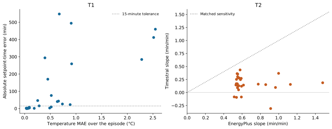
Left: temperature accuracy and timing accuracy can tell different stories. Right: a model that reproduces the simulated response to changed starts would lie near the diagonal.

Second question: does it understand the shifted start?

Across the four nonzero offsets, the mean absolute shift error is 24.4 minutes. In three additional cases, the forecast does not reach the threshold before the horizon ends.

Change in HVAC start	Mean absolute shift error
−60 min	19.6 min
−30 min	10.4 min
+30 min	24.3 min
+60 min	43.0 min

For instance, when we delay heating by an hour, the mean signed shift error at this offset is −43.0 minutes. The predicted comfort time generally moves much less than it does in EnergyPlus. It looks like the model is not capturing the causal effect of the action, even when it has already learned to forecast the usual schedule.

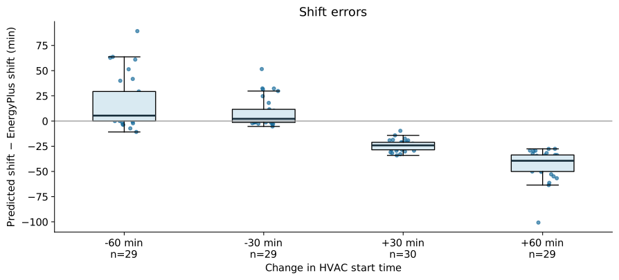
Another way to inspect this is to fit the relationship between start offset and comfort time for each date. The median of the per-date ratios between Timestral’s slope and EnergyPlus’s slope is 0.25. By this measure, the model captures about a quarter of the simulated sensitivity.

Note: we should not expect comfort to move exactly one minute for every minute of start delay. Heat-up duration changes with conditions, and enabling HVAC earlier may have little effect.

Visualizing counterfactual performance

We can explore each date in more detail. The following interactive explorer shows the forecasted and simulated temperature trajectories for a given morning, with the baseline start and four shifted starts. The shaded band shows the pointwise q10-q90 quantiles of the forecast.

The interactive explorer requires JavaScript. Static trajectories: January 12.

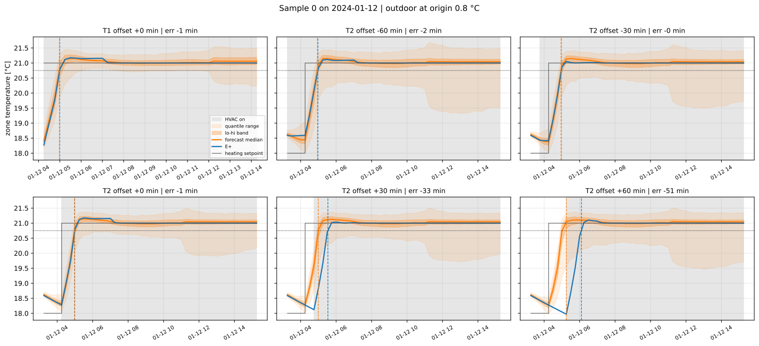
Let’s look at January 12. With the schedule unchanged, the T1 comfort-time error is less than one minute. The unchanged T2 reference, issued earlier, is similarly accurate.

Now we delay the start from 04:15 to 05:15:

January 12	EnergyPlus	Timestral
Comfort time, unchanged T2 reference	04:59	04:59
Comfort time, start delayed by one hour	06:06	05:15
Change in comfort time, before rounding	+66.5 min	+16.4 min

The counterfactual shift error is −50.1 minutes. The forecast already warms the zone while HVAC availability is still zero: at 05:00, it predicts 20.73°C, against 18.05°C in EnergyPlus.

This looks like it’s following a known morning pattern, or relying too strongly on the unchanged setpoint. We would need additional tests to distinguish those explanations. What we can observe is that predicting the usual schedule did not ensure an accurate prediction of the changed one.

The forecast-reveal visualization requires JavaScript. Static trajectories: April 18.

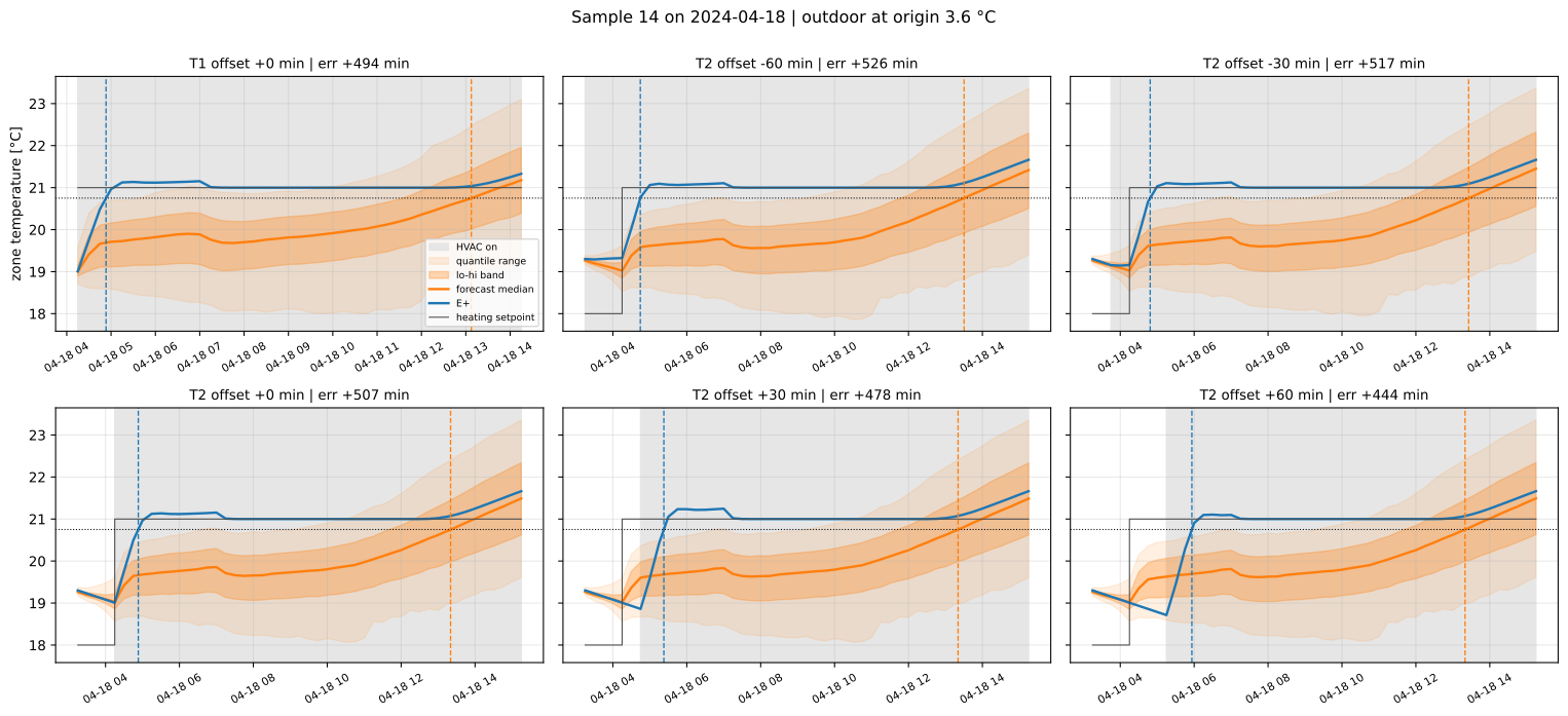
The shaded forecast band shows pointwise q10-q90 temperature quantiles. It helps visualize uncertainty, but should not be read as an 80% confidence interval for the time at which comfort will be reached.

Conclusion

A good zero-shot forecast does not guarantee that the model has learned the causal effect of an action. In our experiment, Timestral-209M often predicts the usual morning well, but underestimates the effect of changing the HVAC start.

Moving from a forecast to a control-oriented model, while staying zero-shot, would then require additional work. However, practical implications become tricky: we don’t want to develop a new model to generate information-rich trajectories for every new building - that’s the opposite of the zero-shot promise. On the other hand, applying excitation techniques to a real building may result in discomfort or wasted energy.

Fine-tuning a foundation model on a small amount of building-specific data may be a more practical way to improve counterfactual accuracy.

References

1. Amria et al. (2026). Time-series Foundation Models for Predictive Control: The Role of Excitation. arXiv preprint.
2. Wang (2026). ThermoForce: A Physics-Structured Interventional World Model for Building HVAC Control. arXiv preprint.
3. Liang et al. (2026). ThermoStill: Distilling Time Series Foundation Model into Thermal Dynamics Model for HVAC Model Predictive Control. ACM e-Energy.
4. Timestral implementation and Timestral-209M model card.