Real world applications of Reinforcement Learning (RL) are still limited as the technology is brittle and requires an enormous amount of simulated interactions. The power of simulated Heating, Ventilation and Air Conditioning (HVAC) systems represent a unique opportunity to use RL in the real systems. Nonetheless, HVAC represent an array of different challenges such as learning robust policies from simulation that can transfer into the real world and defining a reward function that will lead to the desired behavior. In this article, we examine different strategies to deal with the rich action spaces of HVAC systems.

Problem Setting

HVAC systems are complex and made of multiple sub-systems that interact in complex, non-linear ways (see a brief introduction on that in HVAC processes control: can AI help?).

HVAC air and plant loops are responsible for maintaining comfort in buildings occupied zones. Their continuous control is made of a sequence of decisions. Taking the example of an air loop, it can start by deciding how much fresh air the systems lets in, then deciding at what flow rate it must be pushed and at what temperature, and ending with how this air must be “adjusted” for the target zone. Many equipment are involved, like fans, heating and cooling coils, chilled and hot water plant loops, etc.

Let’s build our intuition with a simple example: a heater is equipped with a hot water coil and a fan, and heats the space by controlling the hot water valve and the fan to blow the hot air. If you turn the fan off but keep valve open, hot air won’t move much, and energy consumption will be near 0. If you turn it to maximum position or speed, hot air will move quicker, room will heat quicker too, and energy consumption will be high, both because of the higher fan electricity consumption, and because it increases heat exchange between air and hot water coil.

As a consequence, optimizing control on this simple heating system would require to consider both fan speed and hot water valve position, with prior knowledge that fan and valve have a non-linear dependency regarding temperature of the air blown and energy consumption.

If we generalize this example, many parts of the HVAC system can be seen as dependent to or having a direct or indirect impact on other parts. Trying to control only one equipment as a whole will necessarily lead to suboptimal performance. However, this is often how HVAC systems are controlled: each equipment takes decision regarding a single input. No matter how complex the calculation of this input is, it won’t be differentiable since it’s a single scalar value. Common calculation methods for control decisions rely on linear methods (linear interpolations, PIDs, …) with a narrow view of the state of the system.

That’s where autoregressive (AR) methods and deep reinforcement learning (DRL) can be a good fit: combining function approximation capabilities of neural networks, theoritically unlimited observability of the system and modeling of actions dependencies, the HVAC system and the building it serves could be controlled as a whole (holistic approach), and learned policies could model complex relationships between states and equipment.A

High dimensional action spaces

fig. 1: 3 ways of modeling decision processes with state / action transitions using independent actions distributions (a.) and AR models (b. and c.)

State conditionally independent actions

This is the most common case. In many classic problems, each action of a multi-decision problem is modeled and its probability distribution is estimated as independent from other actions. This doesn’t allow to account for relationships between actions that can be encountered in many problems.

Introducing action dependence with autoregressive policies

Given a policy to optimize with regards to parameters , state , a set of n actions , we can represent the policy as following:

This simple formulation is generic and describes simple relationships and order with action at rank i being dependent on all previous actions.

An example neural network architecture illustrating this formulation is given below

fig. 2: example neural network architecture to model conditional dependencies between actions

In this model, a policy with 2 actions is used. It should be noted that:

• Action 1 and Action 2 are actually parameters of their respective probability distributions (PD).
• Action 1 scalar value (sampled from estimated PD) is passed as input for Action 2 distribution estimation
• Action 1 logits could be passed as input instead of scalar value. This can help preserve information on large discrete/categorical distributions.
• Action 2 inputs could be solely made of Action 1 output (scalar or logits). In such case policy can be formulated as

Note that this model wouldn’t scale well for the estimation of a large number of action distributions. For large action spaces, one can refer to the MADE architecture [1].

Experiments

To validate benefits of such architecture, we compare performance of “classic” network models with the one described in previous section. To draw a fair comparison, the same total number of neural network cells is used in classic and AR policies networks. Furthermore, all other parameters of the Proximal Policy Optimization (PPO, Shulman et al. [2]) algorithm are kept equal between the 2 models.

A path-finding task

The first task is a toy problem where an agent must navigate through a 2D-grid and maximize its reward by moving to certain locations. The action space is designed with 2 actions (vertical and horizontal movements). To emphasize on the need to learn correlation between actions, the reward scheme is modeled using 2 gaussian distributions located on 2 corners of the grid, and a one-time bonus whenever the agent reaches a point close to the mean of each gaussian. The agent starts each episode at the center of the grid. Episode ends when all bonuses are found. We refer to this training environment as bi-modal environment (BME).

fig. 3: rewards distribution over the BME grid

We run 5 experiments with different seeds for each method (classic and AR) on the BME and compare the mean return per episode below.

fig. 4: average episode reward for non AR policy (classic, light green) and AR policy (dark green)

On this toy environment, AR policy achieves a much better mean episode reward than its counterpart.

Visual inspection of trajectories for each method can highlight non-efficiencies and differencies. Below animations capture sample trajectories after 50 training iterations.

fig. 5a and 5b: trajectory examples after 50 training iterations of an agent trained under a classic policy (left) and an AR policy (right)

A simulated HVAC

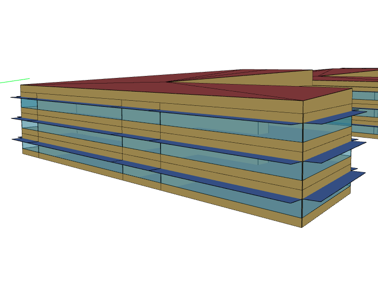
We now use a simulated building and its HVAC. The building model, or digital twin, is created from an actual building and calibrated on Foobot platform using OpenStudio and EnergyPlus open source software. It is a 3 storey office building, with a dedicated outdoor air system, a single air handling unit (AHU) with eletric heating and chilled water coil served by a local plant, and fan coil units for zones comfort.

fig. 6: office building used as a test environment

A policy is trained with and without autoregressive (AR) actions model. The observation and action spaces, reward function, and PPO parameters are identical between the 2 methods. The action space is composed of 2 actions that command the amount and temperature of air supplied to the zones by the AHU. Each experiment is run for 1e6 timesteps.

fig. 7 average episode reward (a., upper left), power demand (b., upper right, in kW), indoor temperature (c., lower left, in Celsius degrees) and CO2 (d., in ppm) for classic and AR policy (blue line) models

AR policy model not only achieves a better mean episode reward (fig 7a.), but it significantly outperforms (by 8.5%) the energy consumption reduction of the classic method. Other reward components, like thermal comfort and indoor air quality, are also better in line with their respective constraints which are a maximum of 25°C indoor temperature and a maximum of 1000ppm for indoor CO2.

Analysing impacts and relationships

To understand better our model, a short study is conducted to highlight how action 1 influence action 2, how each action influence the state space, and what part of the state space has the most influence on agent decisions.

To do that, we’ll first map our system and learned policy with functions approximations that govern it. They can be seen as forward models that predict the behavior of our policy.

• transitions that associates an action and a state to a next state
• rewards that maps action and state with its immediate reward
• policy that maps a state and the next action
• autoregression that looks for correlation between action 1 and action 2

We then compute the jacobian of each function in order to differentiate with respect to relevant parameters. For instance, to highlight what part of the state space is directly influenced by agent decisions, we’ll use the jacobian of the transitions function and differentiate with respect to agent actions.

fig. 8: what part of the state space influences decisions the most, for each action a1 (left) and a2 (right). Actions a1 and a2 seem influenced by different parts of the state

fig. 9: what part of the state space is "controllable" by the policy, for each action (a1, a2) of the space. Here indoor conditions are the most influenced, from both actions

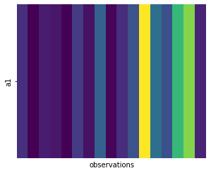
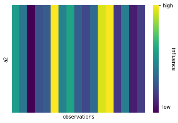
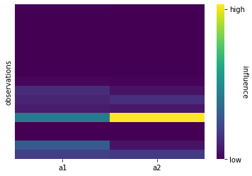
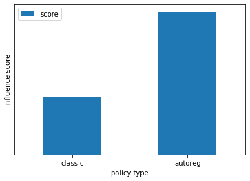
Influence of a1 over a2 can also be estimated thanks to computing the jacobian of the forward model that approximates the predictor function that gives a2 knowing a1. This allows to highlight the much stronger influence score of a1 over a2, as shown in figure 11.

fig. 10: a1 influence on a2, as a scalar score. Left bar for a classic model, right for the AR one

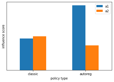
We can also estimate how much each action influence the immediate reward. Interestingly, forward models learned on AR and classic policies lead different estimate: model learned on classic policy shows a somewhat equal influence of each action, while model learned on AR policy shows a much stronger influence of a1.

fig. 11: a1 and a2 influence score on immediate reward, for each policy type

Conclusion

Through a series of examples we’ve demonstrated that autoregressive (AR) policies can bring significant performance and training speed improvements compared to more classic models.

References

[1] Mathieu Germain, Karol Gregor, Iain Murray, Hugo Larochelle. MADE: Masked Autoencoder for Distribution Estimation 2015

[2] John Schulman, Filip Wolski, Prafulla Dhariwal, Alec Radford, Oleg Klimov. Proximal Policy Optimization Algorithms 2017