HVAC processes control: can AI help?
Through a series of examples, this article deals with limitations of classic controllers and control strategies in Heating, Ventilation and Air Conditioning (HVAC) systems, and draws a comparison with intelligent agents (supported by artificial intelligence techniques) and their benefits. As such, we take as a basis of comparison a common HVAC system type (Variable Air Volume or VAV) and show where classic control technics fall short while intelligent agents bring in better performance.
HVAC components control optimization: context
According to US Energy Information Agency, HVAC systems were responsible for not less than 40% of energy consumption in commercial buildings in 2012. With such a significant footprint, everyone has an interest in optimizing their control and operations.
Below diagram gives a simplified description of such HVAC system, of VAV type, as we find in many buildings in US, Europe and Asia since 1980 onwards. This type of system, as its name suggests, varies the amount of air to meet heating, cooling and air renewal demands in building spaces. While its installation cost is higher than previous generation (namely, Constant Air Volume), it has replaced it advantageously since it brings better comfort guarantees and less energy expenses. We encounter this in medium to large size buildings mainly, in every kind of facilities.

As we can observe, a VAV is a centralized system: most of the ventilation, cooling and heating happens in one place, and this requires to be configured and operated to meet all demands. By intuition, one can already imagine the challenges that such systems face: a single (or a handful of) equipment of any kind must satisfy potentially dozens of open spaces, cell offices, meeting rooms, … This requires proper sizing, configuration and control.
To do so, HVAC industry relies on processes, hardware and techniques that, for some of them, are decades-old. Given investment costs to design and promote new equipment or control techniques, but also to replace those already installed, there is some inertia, legitimate to some extent. But as we’ll discuss in next sections, optimisation or removal of existing limitations don’t require many capital expenditure anymore. Modern, software-based approaches can bring dramatic improvements without a full-fledged retrofit.
Shortcomings of classic controllers in HVAC systems
To understand what can go wrong, let’s begin our short study by describing classic control systems and strategies in HVAC systems, backed by concrete examples of sub-optimal control in an actual building.
A classic controller case study: Proportional-Integral-Derivative
Proportional-Integral-Derivative, or PID, are the three calculation terms employed in this type of controller to obtain a process control loop. For many decades, it’s the go-to in industrial processes, and HVAC systems are no exception.
However, they have known limitations, that are common to all PID controllers or more specific to HVAC-related processes. Below we summarize some of them, in order to build a first intuition on what could be optimized.
Typical limitations of a PID
Let’s take an example with an actual PID controller used to vary supply air fan speed in a VAV system. A common control strategy is to make the most-open VAV box damper position reach 90%. So this PID has the maximum of all dampers position as input, a fixed set point of 90%, and outputs fan speed.
The first limitation is intrinsically coming from how PID works: it requires a margin in the set point to produce stable results when the controlled process is mechanical (e.g. fan speed can’t go higher than 100% or lower than 0%). When the limit of process range is reached, errors accumulate but the controlled process can’t go further in the same direction. This is known as integral windup. When it comes to fan control, a typical strategy is then to fix the set point below range limit, usually 90%.
The second limitation is also inherent to PID internals: a large change in set point or in input value will produce excessive change in the output (mostly due to derivative part of the PID: on a large change, derivative term will be very large). A common solution is to use ramping either on set point or on PID input (in some “enhanced” controllers). This produces very slow responses, on a fan start-up that means a long delay before reaching the set point. This can be observed on below chart, where it takes more than 30min for the PID to reach the set point.
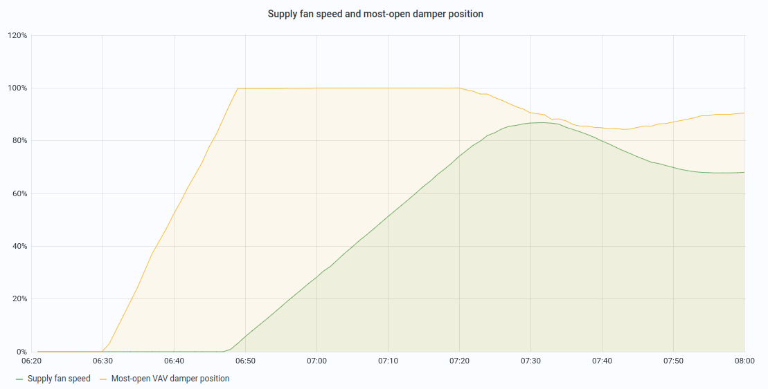
Note: ramping is still necessary to deal with mechanical constraints, a common rule is to avoid changes larger than 10%
per minute on fan speed.
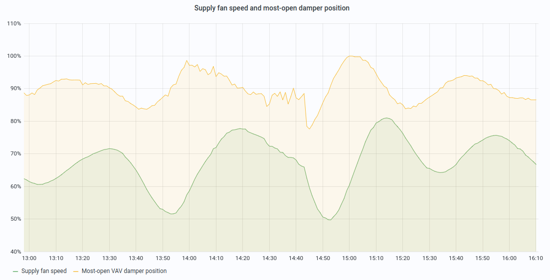
A third limitation comes from PID gains tuning which is a tedious and time-consuming process. Even when controllers come with pre-defined and safe tunings for a particular class of equipment, the HVAC engineer will have to reconfigure them to reach good performance, since each ventilation system is unique. However, this tuning, performed once for all (HVAC configurations are only partially revised from time to time), has about zero chance to cover all operating conditions. This results in typical PID problems like overshooting , oscillations or hunting. This can be observed in chart below, where the desired set point is still fixed at 90%
Last but not least, PID controllers are often driven by a single input: in our case, most-open VAV damper position. However, is this really the goal of a supply fan or did we just find a proxy to accommodate with controller specifications? The actual real goal is to maintain good thermal and air quality comfort in occupied spaces, while minimizing energy consumption.
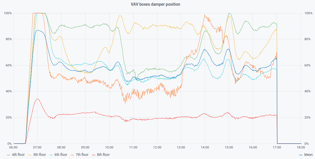
While the proxy target of 90% can satisfy first part, it has no consideration for energy savings. How does this translate? This is very usual to find one damper open at 90% while others are way below. This isn’t just a PID problem (or more specifically, just with the PID controlling the fan), but it’s natural to have zones with less air demand than others, and zones that are almost always in demand (also known as rogue zones). With a PID, one can’t do anything about that. Figure 4 illustrates this problem, where a large difference occurs between damper positions.
“If only I had known that before…”
A PID is only reacting: for a given change in input, it will vary its output to keep as close as possible to its set point. It has no way to anticipate changes or take proactive actions, since it has neither explicit nor inferred knowledge of the controlled system. Moreover, its single input gives it a very partial view of the process at hand.
With such observer model, anticipation isn’t possible, while simple intuitions could be used to save bits of energy here and there. A simple example: when HVAC scheduled end of operations is in sight, one could be tempted to slowly reduce heating or cooling equipment use but not too much to reach end time between desired spaces set points. This is something a PID can’t do.
If we generalise this example, the optimal system should learn building thermal dynamics and discover best control strategies. There are many, and they depend on building use and characteristics.
Design conditions versus reality
As stated in Pacific Northwest National Laboratory report Energy Savings for Occupancy-Based Control (OBC) of Variable-Air-Volume (VAV) Systems:
Each terminal box has a minimum air-flow rate that ensures the ventilation requirements of the occupants of the zone served are met. This minimum air-flow rate is maintained at a constant value based on the design occupancy of the zone, which often corresponds to the maximum occupancy, because measurements of actual occupancy are not currently used to adjust the flow rate. […] In practice, control system integrators and installers often set the cooling minimum air-flow rate for ventilation to between 30% and 50% of the maximum air-flow rate of the terminal box.
The process of Testing, Adjusting and Balancing (TAB) of a building HVAC system is meant to deliver sufficient amount of air, and make sure there will be enough heating and cooling capacity. All the calculation and testing is performed using building design conditions. In practice, it is undertaken when building is still unoccupied, during one or a handful of days (so during a particular season, with specific weather conditions). It doesn’t cover the actual use of the building, which will vary over the course of its life: daily changes - with spaces more or less occupied depending on the hour of the day - and more profound and permanent changes, like when exceptional conditions arise (Covid-19 and its cascade of lockdowns), or simply because tenants’ activity changes.
Another source of HVAC system misconfiguration and excessive energy use is the small and repetitive adjustments made over time by people who are responsible for occupants comfort, or to deal with system instability (operational conditions not tested during initial setup). While it seems natural they make everything they can to guarantee satisfactory living conditions, this often results in more energy wasted due to narrowed operational behaviour (e.g. raising minimum set points).
Non-linearity in controlled systems
HVAC systems are (highly) non-linear: they will respond non-linearly depending on controlled equipment, command magnitude, and current state of the system (for instance: cooling or heating mode).
A classic example can be drawn from fan affinity laws: pressure is proportional to the square of shaft speed. Basically, as fan speed increases, pressure developed by the fan increases twice faster. This is only from a theoretical perspective though, and many factors will add to make this pressure/speed relationship even less linear. What does it mean for a classic controller like a PID? It won’t care, since it has no knowledge of this, and will vary the output without taking into account that it’s already in the high end or low end of the range.
Another example of non-linear system is heat exchanger, that is used in several HVAC components (heat recovery, hot water heating plates, …). Heat exchange efficiency varies depending on the fluid flow rate between which heat transfer occurs. How much heat exchange efficiency is non-linear depends on equipment capacity, often rated using a heat transfer coefficient.
fig. 5: heat transfer efficiency at various flows and T° eff.
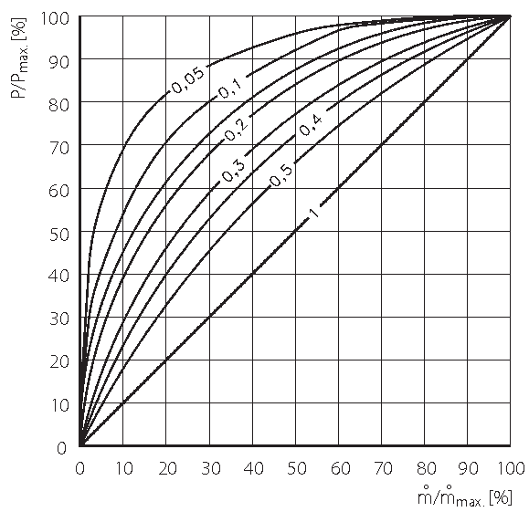
In fig. 5 (reference) , we can see relationship between percentage flow and percentage of heat transferred, for a range of thermal efficiency between 0.05 and 1 (ideal).
Notes:
P/Pmax: percentage of heat transferredm/mmax: percentage flow- thermal efficiency is the ratio between maximum difference in temperature between primary inlet (heating) and
secondary inlet (heated) fluids, and difference in temperature between primary inlet fluid and primary outlet (
returned to heating system) fluids (equation:
ηth = (T11 - T12) / (T
11 - T21)
).
Using a linear controller, like a PID to control for instance a heating valve is thus going to provide a sub-optimal performance.
An HVAC system is composed of many non-linear sub-systems, some interacting together with complex relationships. It is therefore very limiting to use a linear controller to control equipment that responds non-linearly and have interactions on many systems.
Supply Air Temperature (SAT) and the open loop problem
Another common control point in HVAC systems, that is often a target for control optimisation is Supply Air Temperature (SAT). SAT at air handling unit level is commonly controlled using a temperature set point. In general, the set point must be set, so cooled air arriving at the air terminals is cold enough to meet cooling demand (but reheated at terminal unit level when necessary). In humid climate, the set point is often set low so to dehumidify (thanks to condensation) the air and avoid moisture problems.
What do we need to optimise here? SAT set point will have a significant influence on energy consumed by mechanical cooling, reheat and also supply fan. In order to minimize energy consumption, this set point can be varied using a reset strategy (commonly referred to as SAT set point reset strategy).
Why is an open loop a problem?
Although many SAT set point reset strategies exist , it is still very common to find outdoor air temperature-based reset strategy (OA reset) used, even in recent buildings. The assumption is often made, in cold or mild climates that don’t have high cooling loads, a more sophisticated approach wouldn’t worth the pain. It’s only partially true because a too cold air will require more reheat, hence also wasting heating energy. Outdoor air temperature-based reset is an open loop problem: a linear relationship is assumed between outdoor air temperature and need for cooling. In practice, a linear equation computes SAT set point based only on outdoor air temperature, without taking into account the actual indoor conditions, leading to cold complaints problems and high reheat wastes.
Any better yet?
What about more sophisticated strategies then? They are based on heuristics (like the Trim and Respond logic recently
advertised in ASHRAE guideline 36) that vary the set point based on cooling demand: air terminal dampers position
and/or cooling valves position is used as input to compute an increase or a decrease of the SAT set point. While it
brings some indubitable benefits, this has some drawbacks too: such an approach requires thorough tuning and testing (
many variables at stake, like number of ignored requests, thresholds to consider for cooling demand, …) on a
significant period of time (to meet enough variate conditions) and it doesn’t take into account another highly
non-linear aspect: while SAT set point increases to reduce chilled water use, supply fan speed will increase to respond
to unsatisfied cooling needs (if the supply fan speed is variable and also reset, based on static pressure for instance)
.
Hence, supply fan electricity use will increase, but this method can’t tell when increasing SAT set point stops being
advantageous.
As we’ve seen, there are many ways HVAC system operations can drift from their intended performance. We scratched the surface of some challenges HVAC engineers, but also building owners and facility managers, struggle with to keep occupants satisfied while minimising energy consumption of HVAC systems, which accounts in average for 40% of the total building energy consumption. We’ll now see why and how Artificial Intelligence (AI) can bring to help taking back control.
What does AI bring to HVAC control?
For almost a decade now, we find usage of AI in all corners of our digital life: image classification, speech recognition and synthesis, even fake videos generation. A special class of AI technique has drawn attention starting in 2015, called Deep Reinforcement Learning (DRL). It differs from “classic” deep learning techniques in that an agent is trained by interacting with its environment, learning from its mistakes and successes (quantified by a “reward” or a “penalty” given to the agent on every action). It has shown incredible successes with trained agents beating human experts at games like Go or Starcraft, and is used in autonomous vehicles, robotics, and industry.
There are some important, fundamental, differences with other learning techniques that make it particularly attractive for use in process control:
- it can learn in simulated environments, hence data quantity and quality is not a problem. Successful application of deep learning has always been limited by lack of good quality data. DRL does not have this limitation.
- it learns to control: a DRL agent interacts with its environment while trying to maximize the rewards it gets from the actions it performs. This gives it the ability to test, learn and optimise to their best some control strategies that no human could ever discover.
- a domain specialist can encode expert knowledge in the simulated environment and in the reward function to guide the agent towards expected performance. For instance in a multi-objectives problem, one can choose to reward the agent more on one objective than another.
There are many other differences, some of which are specific to current problem at hand in this article. As a matter of fact, HVAC systems are an excellent target for control optimization using DRL, and this is an active topic of research:
- DeepMind demonstrated this on Google data-centers. There are no official numbers, but Google is now using it generally to reduce their energy costs. See for instance DeepMind AI Reduces Google Data Centre Cooling Bill by 40%
- Scientific research on the topic has been very active, as reflects number of papers produced since 2017. A good example of such a paper is Deep Reinforcement Learning for Building HVAC Control
Let’s now detail most important features and compare them with classic HVAC system controllers.
Seeing more than a single input
A DRL agent can be fed with as many environment observations as wanted (only limited by CPU and memory required to train and serve the learned control policy). This means it can “see” current indoor temperatures, outdoor conditions, mechanical and operation status of the system, … Everything that can have an influence of the relevance of its decisions.
This makes a significant difference with a classic controller, that usually takes only 1 input. Even if this input is an aggregation of several observations, this is often insufficient to take an optimal decision. For instance, how to tell the difference between a damper opened because of a heat demand or a cold demand? This can make a significant difference in the response to give, depending on a chiller or a heater operational status, and heat exchange properties.
Learning system dynamics
Every building is unique and has its own characteristics in terms of thermal inertia, systems implementation, or occupancy patterns. More than just learning to cool the air when temperature is high, a DRL agent will learn intrinsic thermal dynamics of the building, and will be able to give a response in the “correct proportion”, without overshooting or undershooting.
A simple example of this is fan speed control with holistic knowledge of the environment state: while PID control strategy described in previous section only looks at most-open damper, DRL agent “knows” about actual thermal conditions and all other dampers positions. It can therefore adapt its response appropriately. If there is only 1 zone in demand, it’s not the same thing as 2 or 3, as a greater air volume is needed as number of zones increases. A PID would have hard time not hunting, and as it would take time to stabilise, the system would already be in a different, transient state.
A benefit of this holistic approach to HVAC control is that one can effectively reduce use of over-sized equipment, or simply configured to run with very defensive set points. When classic controllers give unsatisfactory results when system state is at extremes, or simply during transitions, a DRL agent has learned to deal with them through virtual decades of different, randomised environment conditions.
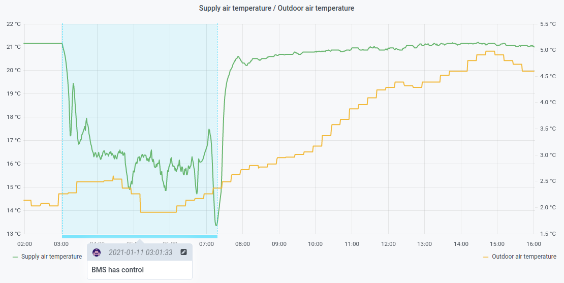
Here is a concrete example of these benefits: a HVAC system equipped with a heat recovery machine saves on heating and cooling energy by transferring sensible (or total, including latent) heat from return air ducts to supply ones. Heat transfer efficiency depends on equipment characteristics and air flow rate: basically, the faster the air moves, the less heat (or cold) can be transferred. A classic controller has no way to take advantage of this property, and will inevitably push more air as heating or cooling demand increases. A DRL agent controlling the fan will learn that minimising air flow will improve heat recovery.
Below graph shows such difference in approach, which leads to a supply air temperature difference of about 5 degrees between classic and AI control.
Anticipation
A DRL agent learns from a reward it gets on every decision it makes. During the training, every action leads to a state of the system, which is used to compute this reward. The purpose of the training (or teaching) is to make the agent maximize the sum of its rewards. So not every single reward separately, but a couple of them. Intuitively, this introduces a very fundamental: we are more interested in the overall result than by each decision taken separately, so the control strategies the agent can discover are very different.
Some concrete examples:
- agent may take decision that seems bad (in terms of instant reward) but that will lead to much better results on consecutive ones. For instance, to minimize power demand when energy price is highest, agent may decide to cool spaces in advance, lowering electricity demand when actual cooling demand should be highest (afternoon).
- along with learned building thermal dynamics, anticipation of HVAC end of operations (when scheduled) can lead to interesting strategies: agent will learn to reduce equipment use by just the right proportion until end time is reached, while maintaining desired comfort. A classic control would just push things as usual, as it has no knowledge of thermal dynamics or schedules.
Anticipation, as an inherent feature of reinforcement learning, also brings a difference with other AI and deep learning techniques like forecast. In time series forecast, a model is trained to predict next few minutes or hours of one or more variables given some observations. This can be used to predict, for instance, what the indoor temperature will be given past indoor, outdoor and system conditions. With such technique, each decision goes isolated from each other, and there is no simple way to build strategies that span multiple control steps.
Testing hypotheses and strategies in days, not months
When a building HVAC system requires a partial or entire retrofit, the project takes from several months to years before achievement. As it involves hardware changes, and very important expenses, an energy performance audit is conducted to assess current building strengths and weaknesses, and prescribe upgrades that would be the most cost effective (depending on goals, but return on investment is often key).
This is where simulation can take place: using a detailed building model, calibrated against historical energy consumption, auditors can test various scenarios and simulate their efficiency. It offers a way to make educated, data driven decisions, and not relying only on experience. The exact same basis can be used to train a deep reinforcement learning agent to control HVAC equipment: since the building model that serves as training environment is calibrated, not only the agent is learning from a realistic environment, but its achievements and performance will have solid ground.
Figure 7 shows an overview of a digital twin acquisition process (calibrated building model) used to train deep reinforcement learning agents to obtain optimal HVAC control policies, that can be later deployed to control actual building HVAC system.
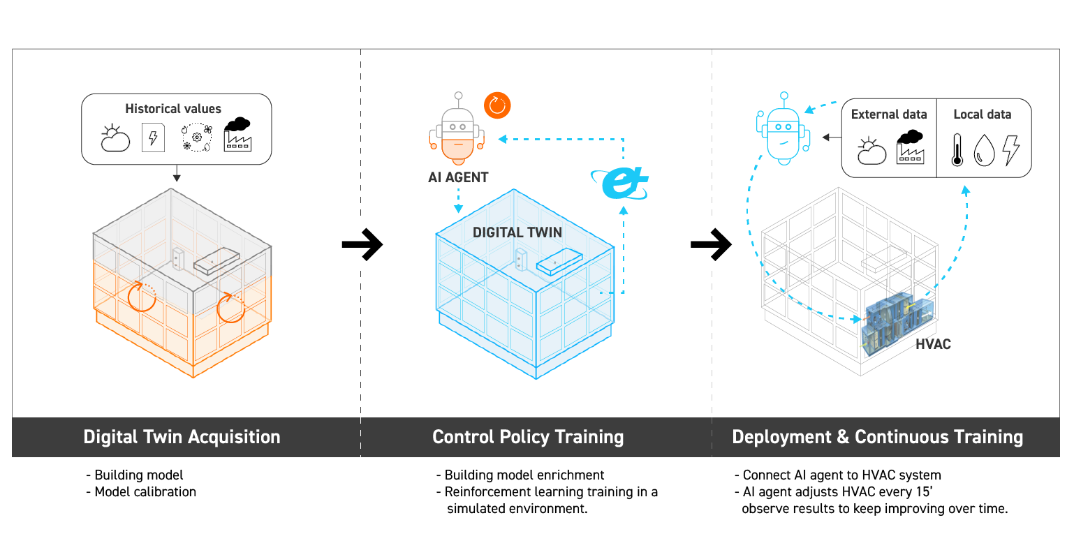
The comparison with classic retrofit projects stops here though: when it will often take months or even years to finalize an HVAC hardware upgrade, a DRL control policy can be deployed in days. Apart from the obvious improvement in duration, such work-flow is a real plus for building owners and property managers, since it relies on:
- a clear and standardised modelling and calibration process (e.g. calibration is backed by ASHRAE guideline 14)
- a cost-effective simulation process to test strategies
- an additional and valuable asset (the building model itself) that concentrates all necessary information about the building, for present and future projects
Simulation engines, as a source of training data for deep reinforcement learning, have other key benefits compared to other solutions:
- they produce an infinite stream of data of excellent quality (historical data can be sparse, noisy, hard to interpret and parse, sometimes unusable)
- they give a holistic view of building conditions: you can simulate indoor air quality (rarely available in building historical data), randomized conditions, etc.
- agent can be prepared to worst case scenarios: extreme weather, HVAC faults, … Something that is hard to get otherwise.
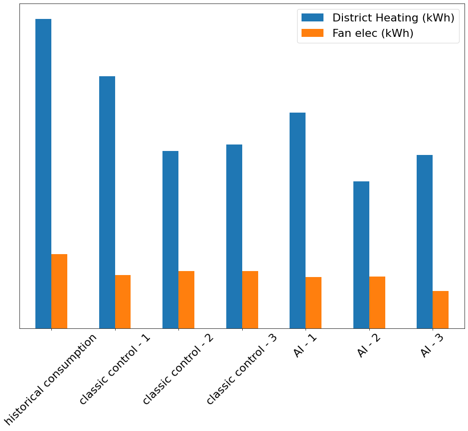
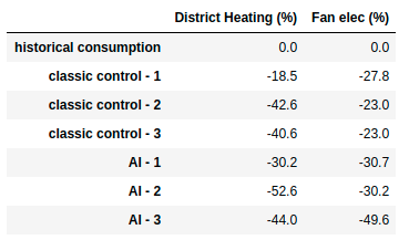
Figures 8a and 8b illustrate HVAC optimization proposals one can easily test in a couple of days using a calibrated model and DRL.
There’s also a clear difference with forecast-based techniques, which can only rely on historical data from the building. Historical data from Building Management System (BMS) or other sources is often scarce, if ever present. With scarce data, you are limited to what the model can learn from, so the number of potential strategies will be small. If you don’t have enough data, the only thing you can do is… wait! Several months at least, because the model needs to be trained on different weather conditions to produce satisfactory results. Imagine you collect only data during summer, what happens in winter when the model is proposed with unseen conditions is likely to be arbitrary decisions. If we generalize, it’s very likely that a forecast model will take years to be self-sufficient, the time it takes to collect enough data.
Additional benefits
Something that is harder to quantify, but has reasonable logical ground, is that making control more stable increases mechanical equipment lifespan. By anticipating needs and taking only one action every few minutes, AI can help avoiding turning equipment on and off constantly, but most importantly solves poor programming control logics.
Taking fan speed control as an example, we saw already in previous examples some diseases a fan can suffer from, like large oscillations throughout the day, likely because of its controller characteristics but also due to how its input varies: static pressure reset or most-open damper control strategies can bring instability. As a result, the fan speeds up and slows down throughout the day, wasting energy in acceleration and deceleration, some of which is simply expelled as heat. This added to the constraint supported by the fan belt, will eventually decrease fan lifespan.
On the other hand, AI, thanks to its anticipation capability, doesn’t need to constantly react to changes in input. With a multimillion time steps training, and practical training constraints, a reinforcement learning agent learns to keep control stable and to avoid large changes. HVAC equipment, with thousands of dollars cost for each piece, is preserved longer.
Results in an actual building
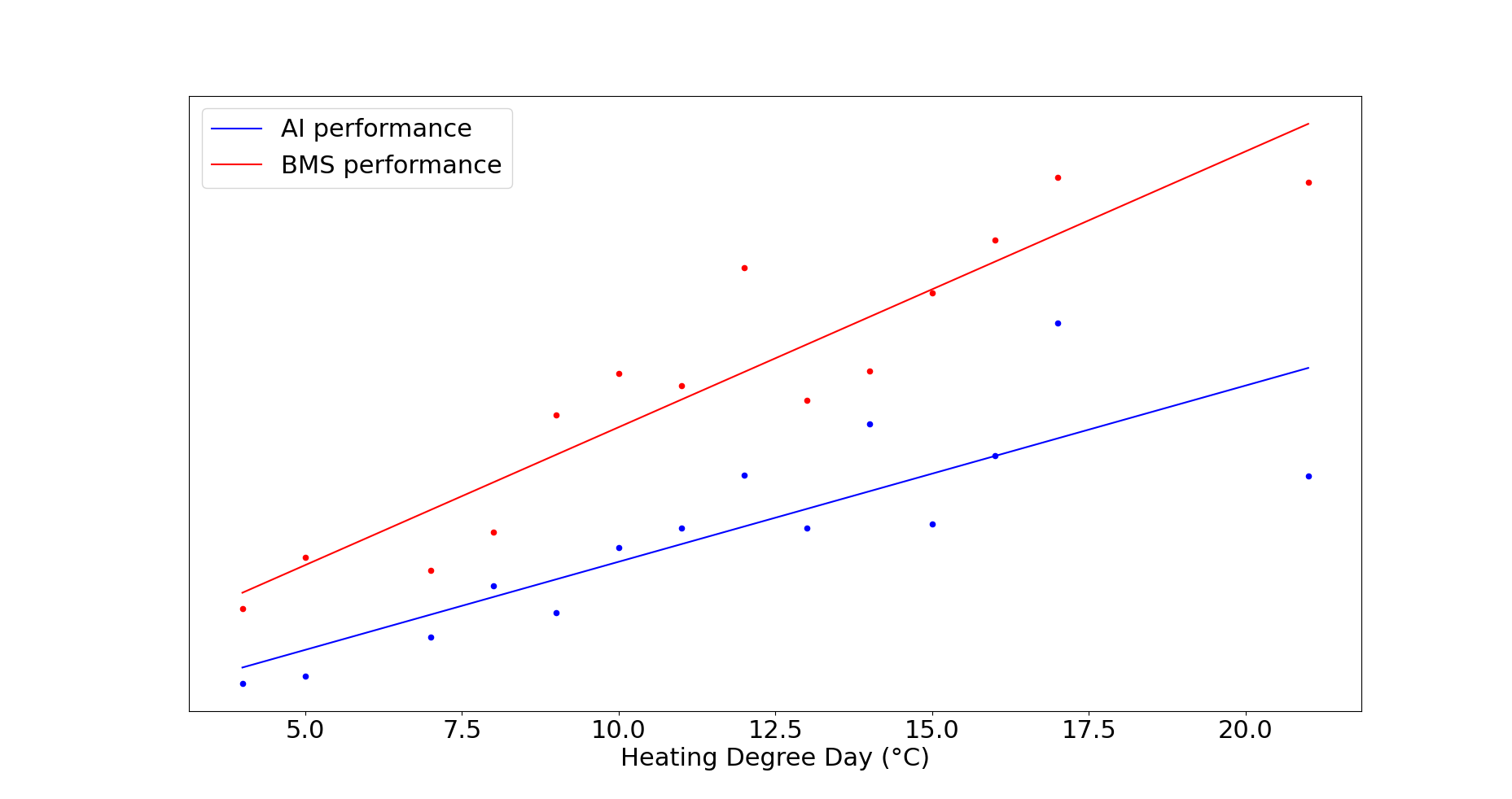
Above chart shows results obtained by multiple deep reinforcement learning agents that took control of HVAC equipment in an actual commercial building. From day 1, they have been efficient and proved to adapt well to changing conditions. Taking denormalized results on this 3 months period (100% of the period), they obtained 47% savings in $ compared to previous years utilities bills data. Using normalized results (typical office hours), savings were up to 65%.
Conclusion
In this article, we’ve seen how artificial intelligence, and deep reinforcement learning in particular, is well suited for HVAC control optimizations. With a cost-effective and robust process based on building models, calibration and teaching in simulated environment, efficient control policies can be discovered to achieve significant savings.