Introduction

Off-Policy Policy Evaluation (OPE) is a technique for estimating the performance of a new reinforcement learning policy ($\pi_e$) using historical data collected from a different behavior policy ($\pi_b$). This approach enables policy comparison and selection without deploying new policies into production, reducing risk and cost.

OPE relies on the mathematical framework of importance sampling and model-based estimation to provide unbiased or low-bias estimates of policy performance under specific assumptions.

Under importance sampling, the value of the target policy $\pi_e$ can be estimated using trajectories collected under the behavior policy $\pi_b$ as follows:

$V_{\pi_e} = E_{\tau \sim \pi_e}[\sum_{t=0}^T r_t] = E_{\tau \sim \pi_b}[\sum_{t=0}^T \frac{\pi_e(a_t|s_t)}{\pi_b(a_t|s_t)} r_t] \approx \frac{1}{N} \sum_{i=1}^N \sum_{t=0}^T \frac{\pi_e(a_t^i|s_t^i)}{\pi_b(a_t^i|s_t^i)} r_t^i$

Under model-based estimation, a model of the environment is learned from the data collected under $\pi_b$, and then used to simulate trajectories under $\pi_e$ to estimate its performance.

See Hopes library documentation for more details on the mathematical background and different estimators.

OPE is particularly valuable when:

• Deploying untested policies could have negative consequences (safety, costs, user experience)
• We want to evaluate multiple candidate policies before committing to one
• We have sufficient logged data from past deployments

This document explores when OPE is applicable, which estimators to use, how to interpret results, and what alternatives exist from our experience in the field of HVAC control.

When does it make sense?

The applicability of OPE depends on the specific problem, the available data, and the policies being evaluated. Here are some key considerations.

IPS estimators

If $\pi_b$ is deterministic, estimators of the Inverse Propensity Score (IPS) family will fail since $\pi_b(a|s)$ is used as denominator in most definitions. Adding a $\epsilon$ to avoid division by zero introduces bias, and dividing by a small number will make variance blow.

⇒ No IPS if $\pi_b$ is deterministic.

Some IPS estimators also tend to be more prone to high variance due to their definition. For instance, trajectory-wise importance sampling (TWIS) is defined as:

$V_{TWIS} = \frac {1}{n} \sum_{i=1}^n \sum_{t=0}^{T-1} \gamma^t w_{0:T-1}^i r_t^i$

Where importance weight

$w_{0:T-1}^i=\prod_{t=0}^{T-1}\frac{\pi_e(a_t \vert s_t)}{\pi_b(a_t \vert s_t)}$

And $a$ is the action, $s$ the state, $T$ the episode length, $t $$t$the timestep, $\gamma$ the discount factor, and $r$ the reward.

So importance weight is a product over the entire trajectory, with intuitively the following consequence when horizon grows and probabilities mismatch: the product grows or shrinks exponentially, and variance explodes. We found that it can give very unstable results.

In such situation, we prefer per-decision IS-type estimators, which reweights rewards up to a step only.

Direct method

Direct Method estimator uses a learned model of cumulative rewards to estimate policy value. At its core, we use $V^{DM}(s_0) = \sum_{a} \pi_e(a|s_0)·Q(s_0,a)$ for a given episode to estimate future policy return. Since $Q$ is learned from data logged under $\pi_b$, the following assumptions hold:

• if $\pi_b$ and $\pi_e$ have very different responses (actions distribution), it’s very likely that $Q$ will be biased.
• if $\pi_b$ never explores region where $\pi_e$ operates, it’ll be biased too.
• if episodes horizon is long, there is more chance for error to happen and compound.

A possible way to decrease bias for the learned model is to split long episodes into smaller, regular ones, and learn a separate model for each time bucket. While not solving the coverage problem, it can decrease errors due to temporal extrapolation, and makes changes in action distribution more explicit.

Another way to improve results, and this time coverage, is to form a dataset under multiple offline / online policies. For instance, using evaluation data generated during training (when model-based, the bias can then come from system dynamics that don’t match real world system), or by different versions of the behaviour policy.

What estimators can be used, and prerequisites?

IPS estimators

Most IPS estimators use $\frac {\pi_e(a|s)}{\pi_b(a|s)}·r$ as a manner of re-weighting rewards obtained under $\pi_b$. This assumes we need to log following information under $\pi_b$:

• states
• actions
• actions probabilities (propensity scores) → they can’t be reconstructed from logged actions alone by rolling out the policy.
• rewards

In practice, this information should be logged by the policy server (preferred), unless all these information is returned by the policy server and in this case the client side could log it.

We also need $\pi_e$ to be available so we can evaluate action probabilities under this policy. This should be in the shape of the policy model itself, or a probability function that expresses the policy correctly.

Since $\pi_b$ is the denominator, we also need support (coverage), expressed as $\pi_e(a|s) > 0 \implies \pi_b(a|s) > 0$. Which practically means:

• all state - action pairs visited under $\pi_e$ should have been visited under $\pi_b$.
• for all state - action pairs visited under $\pi_e$, the probability of taking the action should never be 0 under $\pi_b$.
• $\pi_b$ shouldn’t be deterministic.

(see also “When does it make sense”).

Direct method

DM assumes learning a model that can predict cumulative return from an initial state, which can perform well across both policies. This assumption usually doesn’t hold, especially if $\pi_b$ and $\pi_e$ have different origins (e.g. very different modeling approaches), or when a new policy is supposed to perform better by taking trajectories unseen under old policy. DM should then be used with caution, by first performing a thorough analysis of the states and actions distributions under the two policies (see also “When does it make sense”).

Compared to IPS, we don’t need logged action probabilities (propensity scores) under $\pi_b$. The rest holds.

General requirements

• Positivity of the reward: this is necessary when confidence interval and lower bound estimates should be computed. This may require to rescale the logged / computed reward, for instance using a MinMaxScaler to obtain a $[0, 1]$ range.
• Reward design consistency: make sure reward function doesn’t change over time, which is often the case in early experiments. OPE might more be adequate when training and deployment workflows are stable.
• Data logging pipeline robustness: as indicated above, there are quite a few things to log, some of them are easier to get than others. When having episodes of length greater than 1, having a field to easily identify them can be interesting (or a done column).
• Finite variance assumption: with long horizons, or slight probability mismatch, variance may explode. In this case, prefer per-decision estimators and / or self-normalized ones.
• Stationarity: if environment is unstable (e.g. in HVAC control depends on weather, occupancy, etc) it can be interesting to segment the analysis by control context to better understand where a new policy works better than another.

How to make sense of the value?

OPE estimators are often biases or have high variance. Well, nothing new, there’s always a trade-off. Except here estimators can be largely biased, and variance can explode easily. Knowing that, how to interpret the output of our estimators? When to trust them?

Good practices

At its core, OPE uses policies values as scores. Policies values are nothing but cumulative sum of rewards over a trajectory, obtained with different manners depending on the estimator.

As a consequence, if rewards, and more importantly their cumulative sum, are easily interpretable (e.g. cases where there is a single term, or equal weights for each term, no scale differences, etc), then we can give an interpretation about the scalar value of the OPE output.

Otherwise, the values should be interpreted by comparison, as in $V(\pi_e) >= V(\pi_b)$, which would mean the cumulative sum of rewards under first policy is higher than under second.

However, comparing values can be a weak estimator (single value comparison, suffering from estimators biases and variances). It’s important to rely on:

• confidence intervals (lower and upper bounds) for the estimators.
• multiple estimators outputs.

For instance, checking if $LB(V(\pi_e)) >= LB(V(\pi_b))$ with $LB$ the lower bound of the confidence interval. It offers stronger guarantees about first policy being “better” than second.

Note that, in all cases it’s possible to:

• output policy value estimates for both $\pi_e$ and $\pi_b$. The first is obtained with OPE estimators, and the second is simply the cumulative sum of rewards under the same trajectories. In practice, we can even run OPE estimators with $\pi_e = \pi_b$, some terms will cancel.
• estimate multiple policies values to take a decision, e.g. $\pi_e^i \in P$ where $P$ is an ensemble of available target policies.

Beyond good practices, understanding data at hand

There are several practical things to consider about the dataset and the problem at hand which may lead to different interpretations of the results:

• Reward representativeness: does the reward truly capture the operational objective? In real-world problems, this isn’t always the case, because of missing information for reward design that is replaced by shaping. Sparse or delayed rewards are particularly difficult to handle, especially for trajectory-wise estimators: for instance Direct Method is only as good as the Q model it relies on, for which a new trajectory might be out of distribution. Consider careful inspection of reward distributions, using multiple estimators, splitting episodes into representative subsets, and introducing time or step information observations.
• Reward scale and variance: high reward variance increases estimator variance. It requires dealing with outliers steps or episodes (pruning), re-scaling rewards, and using robust estimators.
• Action space shape: special care needed when action imbalance exists. This leads to numeric instability of weights under IPS estimators, and estimators using a Q model may never see some actions taken under $\pi_b$.

Going in production: How to handle overridden policy decisions?

In real-world systems policy decisions can be overridden by safety rules, manual decisions, etc. This comes as a challenge for OPE as the logged propensities under $\pi_b$ no longer match the actual action applied, resulting in state and reward not being the result of the policy decision.

A concrete example is the HVAC equipment optimal start problem we tackle with RL: we can frame it as a sequential decision problem, where the policy decides at each step if equipment must be switched on. Once the policy has decided to switch on the system the first time, an “action stickiness” mechanism applies to keep the equipment turned on (both during training and real-world inference). This comes as a challenge for many estimators, like IPS-style estimators:

• $\pi_b(a|s)$ can still tell action 0 is more likely, but the state and reward will be the one obtained by taking $a = 1$.
• The estimator become biased as we will basically reweight the reward of taking $a = 1$ with the probability of not taking it.
• Cumulative sum of rewards must be computed until end of episode as states and rewards after the initial switch time are important: the verification of the achievement is delayed and compounds as policy is penalized at every step for taking an action early and penalized for not achieving comfort at specific time (end of episode). So we can’t truncate episodes until first switch on time.

A first naive solution

Here are 2 practical solutions that differ in implementation but eventually end up to the same result:

1. Correct propensities by integrating the action stickiness information as an augmented state $s’ = (s, z =\text {switch has happened})$. For both $\pi_e$ and $\pi_b$, we should have $\pi(1|z=1) = 1$. This guarantees support and no division by zero.
2. Consider the episodes as 2 sub-episodes, the first part where propensities are applied until first switch time, the second where only reward is kept as the importance ratio cancel with $\frac {\pi_e(1|s) = 1}{\pi_b(1|s) = 1} = 1$

The first option could be cleaner, and could be used for all kind of IPS-like estimators. However, there are 2 important caveats to understand:

• this solution only holds if action stickiness applies to both policies.
• this solution introduces a bias as it hides what could happen if $\pi_e$ can decide to switch on later than $\pi_b$: by forcing the same action probabilities on both policies at the timestep where $\pi_b$ decided to switch on, we don’t take into account the possibility of $\pi_e$ deciding to switch on later. Same applies if it’s possible for $\pi_e$ to switch on earlier than $\pi_b$.

As a consequence, this first solution (both options) will only highlight the difference between policies in the first part of the episode, and not in the second part where the achievement of comfort is verified. This can be a problem if we want to evaluate policies on their ability to achieve comfort, which is often the case in HVAC control.

Below is an illustration of the problem and the naive solution for a single episode:

Illustration of the problem of overridden policy decisions for OPE. The behavior policy $\pi_b$ is supposed to take action 0, but action 1 is applied instead, leading to a mismatch between logged propensities and actual rewards.

Reshaping the problem

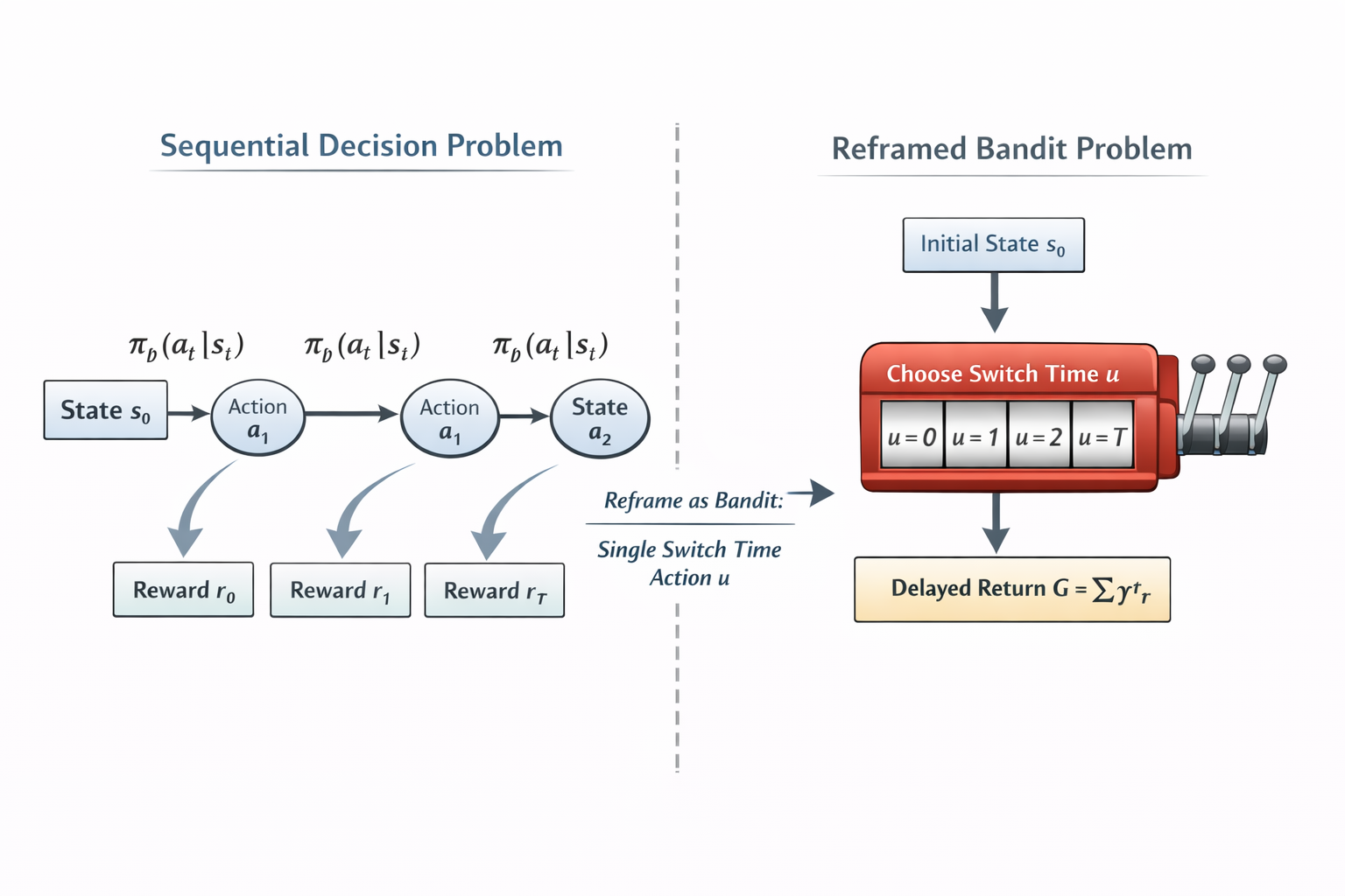
The initial problem is a sequential binary-action decision process. It is possible to reparameterize the sequential decision problem into a single episodic action corresponding to the switch time. Instead of modeling the sequence of binary actions, we treat the episode as choosing one decision variable $u$ representing the timestep at which the switch occurs.

Let’s consider:

• $s_0$ the state which carries information about the initial system state, the objective, and forecast data.
• $u \in U = {0, 1, …, T}$ the new single action per episode (bandit) which states only at what step the switch-on occurs, for instance $u = 4$ means switch on happens at timestep 4 in the original problem setting.
• $G = \sum_{t=0}^T \gamma^t r_t$ the whole episode return.

We now reformulate the new propensity $\pi^z$ under this reframed problem as the probability for the policy to switch on at $u$. This can be defined as:

$\pi^{z}(u, s_0) = (\prod_{t=0}^{u-1} \pi(0 \vert s_t)) \cdot \pi(1 \vert s_u)$

Above equation can be read as the product of probabilities for taking action 0 (keep system off) before timestep $u$ multiplied by probability of taking action 1 (switch on) at step $t = u$.

Although this resembles a contextual bandit formulation, the action propensity still depends on the sequence of intermediate states produced by the sequential dynamics. The bandit action probability is therefore computed as the trajectory probability of switching at time $u$ under the original policy.

Illustration of the original sequential decision process (left) and then reframed as contextual bandit-like problem (right). Image generated by ChatGPT 5.3.

Using an appropriate estimator for this class of problem like IPS, we can now define the value estimate of evaluated policy as:

$V_{IPS} = \frac{1}{n} \sum_{i=1}^n \frac{\pi_e^z(u^i \vert s_0^i)}{\pi_b^z(u^i \vert s_0^i)}G^i$

This is a bit twisted, since we need data from the sequential decision process such as states and action probabilities from both $\pi_b$ and $\pi_e$, while reframing as a single step problem. It offers the advantage of avoiding some support problems we had before, but not all: since we rely on logged switch-on time $u$, if behavior policy doesn’t explore much (e.g. it always starts late in the episode) we may have timesteps not covered by the estimator.

Post-deployment evaluation

As with any continuous deployment technique, continuous monitoring is necessary as a post-deployment evaluation step. This will allow to make sure deployed policy outcome is the desired one. The good thing here is that we won’t rely only on the reward, but on every data available from the target system.

One potential technique, given enough data, is an evaluation based on control-context equivalence (CCE): gathering periods with “similar” context prior and posterior to new policy deployment will allow to make sure the new policy is actually doing better.

Below example shows control-context equivalent evaluation on an optimal start problem:

Bubble plot showing the post-deployment performance of old and new policy evaluated under CCE.

Of course, it’s still possible to rely on OPE, and to compute reward estimates based on logged data after deployment, then compare $\hat{V}(\pi_e)$ with $V(\pi_e)$ with $\hat{V}$ being the value estimated on logged trajectories.

What alternatives exist?

OPE requires to proceed with care and has many pitfalls. It’s easy to fall into traps or regions where the method can’t cover our needs.

Alternatives include:

• using a model of the environment (probabilistic, physics-based twin, etc) to evaluate both policies. This would offer robustness and coverage (any type of policy can be used), but it’s sometimes not available and it’s harder to put in practice (need to run the model with a simulation engine, hook into it to rollout the policy, etc). It introduces a bias:
  • in assuming model accurately captures transition dynamics of the environment, e.g. $\hat{p}(s’|a,s) \approx p(s’|a,s)$
  • in assuming trajectories can be replayed deterministically for the behavior policy $\pi_b$, which might not always be true (e.g. exploration is enabled under $\pi_b$).
• post-deployment policies comparison with control context equivalence (CCE): if both $\pi_b$ and $\pi_e$ have been deployed, comparing their performance can be done if context equivalence can be ensured. As with previous point, we can not only compare their value estimate, but also check their performance in details (per-goal). It also introduces a bias (full equivalence is impossible), and is only possible in an online manner ($\pi_e$ has to be deployed) which reduces its applicability (we often want to estimate performance without deploying).
• online A/B testing: online A/B testing consists in deploying the candidate policy $\pi_e$ to a fraction of traffic while keeping the current policy $\pi_b$ on the remaining traffic, then comparing their outcomes under the same reward definition and operational constraints. Online A/B testing is best used once offline screening (OPE or simulation) suggests a candidate is safe, and when monitoring and rollback mechanisms are in place.

Comparison of the approaches:

Method	No deployment?	No model?	Handles long horizon?	Main risk
OPE	✅	✅	⚠️	bias/variance
Simulator	✅	❌	✅	model error
Online A/B	❌	✅	✅	operations
CCE	❌ (not simultaneously)	✅	✅	context mismatch

Conclusion

OPE is a powerful technique for evaluating policies without deployment, but it requires careful consideration of the problem, data, and estimators used. By following best practices and understanding the limitations, practitioners can make informed decisions about when and how to use OPE effectively. Always consider alternatives and complement OPE with post-deployment monitoring to ensure the best outcomes.

In a future article, we will share more on our experience with OPE in the field of HVAC control, including results obtained on real-world problems.

References

Eligibility traces for off-policy policy evaluation
Intrinsically Efficient, Stable, and Bounded Off-Policy Evaluation for Reinforcement Learning
The Self-Normalized Estimator for Counterfactual Learning
A Review of Off-Policy Evaluation in Reinforcement Learning
Doubly Robust Policy Evaluation and Optimization

Tools

HVAC optimisation with Off Policy Evaluation and Selection