In real world problems, data is often scarce and noisy, limiting how fast an ML/AI-based solution can become effective in the field. Mathematical models of physical phenomena exist, but they require intractable computation times and level of details about the environment.

Physics-informed neural networks (PINNs) were recently introduced as an elegant and efficient way to mary the best of both worlds:

• learn from the theoretical model represented by a partial differential equation (PDE), to ensure robust predictions and limit amount of field data to collect
• learn from field data to adapt the trained neural network to the target environment

This article deals with how well a PINN can solve the well-known heat equation and shows that it could become an enabler for many real-world applications that are currently too complex to solve with deep learning.

PINNs, an overview

Many physical aspects of our surrounding world can be described using PDEs. But computing the solution to these equations often require complex models and details about the environment that are often not available. Worse, solutions would need to be recomputed for every change in the PDE conditions, which will always happen. Depending on the variability of the environment, the number of computations would grow exponentially.

Physics-informed neural networks [1][2] offer an elegant and flexible solution to solve PDEs in a more universal manner:

• thanks to the capacity of neural networks to approximate arbitrary functions, they can also approximate PDEs involving derivatives of different orders
• they are not limited by discretization like classic approximators of PDEs, thus can infer any point in space
• they are not limited to specific boundary or initial conditions, given that they are appropriately trained (ie conditions given as input)
• they take advantage of modern deep learning frameworks auto differentiation methods to compute derivatives (ie torch.autograd)

In this article we’ll see how we can solve the 2 dimensional heat equation.

The Heat Equation, a Partial Differential Equation

Heat diffusion equation [3] describes the diffusion of heat over time and space. It’s a PDE, involving time and space derivatives. The basic equation in a 2D space is:

$$ \begin{equation} \frac{\partial u}{\partial t} = \alpha \frac{\partial^2 u}{\partial x} \frac{\partial^2 u}{\partial y} \end{equation} $$

Note: it’s often simplified using notation $ u_t = \alpha \cdot u_{xx} \cdot u_{yy} $

where $u$ is the function that associates $t, x, y$ with a temperature, $x$ and $y$ points on the 2D surface, $t$ the time variable and $\alpha$ the coefficient of diffusion.

A PDE is also defined by its boundary and initial conditions. In present case we’ll set left, bottom and right edges as cold surfaces at 0 unit of temperature, while the top is heated at 1 unit of temperature:

$$ u(t, 0, y) = u(t, x_{max}, y) = u(t, x, 0) = 0, \text{with} \space 0 \leq y < y_{max} $$ $$ u(t, x, y_{max}) = 1 $$

As an initial condition, we’ll consider the whole surface at 0 unit of temperature, ie $u(0, x, y) = 0$.

Solving with Finite-Difference Method

The Finite-Difference Method (FDM) offers a way to numerically solve PDEs using discrete space and time spaces to enable derivative functions approximation that we saw in $(1)$.

First and second order derivatives can be approximated with

$$ \begin{equation} \frac{\partial u}{\partial t} \approx \frac{u_{i,j}^{k+1} - u_{i,j}^{k}}{\Delta t} \\ \frac{\partial^2 u}{\partial x} = \frac{\partial}{\partial x} \cdot (\frac{\partial u}{\partial x}) \approx \frac{u_{i+1,j}^{k} - 2u_{i,j}^{k} + u_{i-1,j}^{k}}{\Delta x^2} \end{equation} $$

If we transform the whole original equation $(1)$ using $(2)$, we get:

$$ \begin{equation} \frac{u_{i,j}^{k+1} - u_{i,j}^{k}}{\Delta t} = \alpha (\frac{u_{i+1,j}^{k} - 2u_{i,j}^{k} + u_{i-1,j}^{k}}{\Delta x^2} + \frac{u_{i,j+1}^{k} - 2u_{i,j}^{k} + u_{i,j-1}^{k}}{\Delta y^2}) \end{equation} $$

Taking $\Delta x = \Delta y$ (a grid with steps of equal size in all directions), we can simplify the equation to:

$$ \begin{equation} u_{i,j}^{k+1} = \gamma(u_{i+1,j}^{k} + u_{i-1,j}^{k} + u_{i,j+1}^{k} + u_{i,j-1}^{k} -4u_{i,j}^{k}) + u_{i,j}^{k} \\ \text{with} \space \gamma = \alpha \frac{\Delta t}{\Delta x^2} \end{equation} $$

$(4)$ can be quickly implemented using a 3 nested for loops in python, or you can go for a more efficient method using Jax and its Just In Time (JIT) compiler:

delta_t = 0.01
delta_x = 0.1
gamma = alpha * delta_t / delta_x ** 2

@jax.jit
def compute_next_k(u_k):
    next_u = jnp.array(u_k)

    u_next_k = gamma * (
            jnp.roll(u_k, 1, axis=0) +
            jnp.roll(u_k, -1, axis=0) +
            jnp.roll(u_k, 1, axis=1) +
            jnp.roll(u_k, -1, axis=1)
            - 4 * u_k
    ) + u_k

    return next_u.at[1:-1, 1:-1].set(u_next_k[1:-1, 1:-1])

Solving with PINN

Using PINN, we don’t explicitly solve the equation anymore, but it will be used to compute the loss during the training of the neural network. Specifically, the loss will be computed against the derivative of the PDE, and the boundary and initial conditions. In our present case, our loss $L_{eq}$ can be defined to minimize residual of the predicted heat equation $(1)$

Given that we want $ u_t - \alpha u_{xx} u_{yy} = 0 $, the loss can be obtained with

$$ L_{eq} = \frac{1}{N} \sum_{i=1}^{n} \| u_t^i - \alpha u_{xx}^i u_{yy}^i \|^2 $$

Similarly, residuals for boundary (BC) and initial (IC) conditions can be defined as

$$ L_{bc} = \frac{1}{N} \sum_{i=1}^{n} \| u(t, x^b, y^b) - u_{bc} \|^2 $$ $$ L_{ic} = \frac{1}{N} \sum_{i=1}^{n} \| u(0, x, y) - u_{ic} \|^2 $$

The total loss is then:

$$ L_{pde} = L_{eq} + L_{bc} + L_{ic} $$

PINN reveals to be a tractable solution because derivatives computation can be delegated to deep learning frameworks we use to train neural networks: auto differentiation technique is already implemented, so we’ll use it for both back-propagation but also to compute $L_{pde}$.

An example of using pytorch to compute $L_{eq}$:

from torch.autograd import grad
# where u is the neural net module we train, so here we actually perform a forward pass
u_value = u(t, x, y) 
# diffusion coefficient
alpha = 0.1

def _grad(out, inp):
  return grad(
      out, 
      inp, 
      grad_outputs=torch.ones_like(inp), 
      create_graph=True
  )[0]

loss_eq = (
  _grad(u_value, t) 
  - (
    alpha 
    * _grad(_grad(u_value, x), x) 
    * _grad(_grad(u_value, y), y)
  )
)

Results

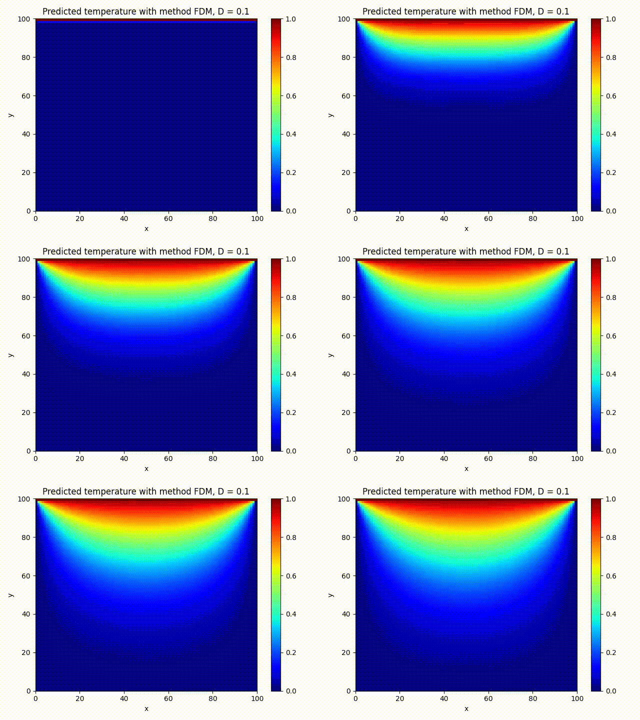
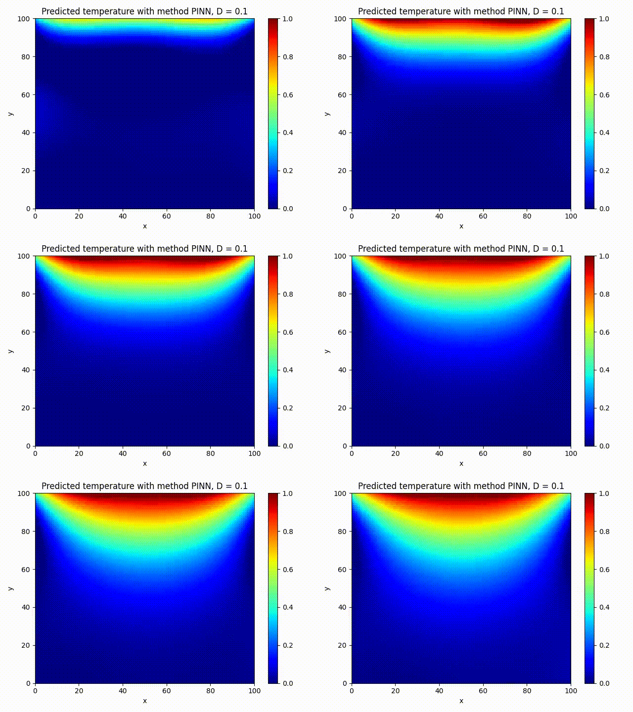
We train a small PINN on 2000 epochs and compare visually against FDM method:

The PINN solution looks very close to the FDM one, that’s what we wanted!

Real world applications

Given that PDEs can be used to model a lot of problems, there are many possible real-world applications for PINNs. Looking for recent papers exploiting them is sufficient to imagine the number of potential new AI-based solutions that may become practical.

With PINNs, it becomes possible to quickly create efficient industrial controllers, starting with minimal amount of field data. When field data is available, training loss can be computed as $L_{total} = L_{pde} + L_{data}$. As more and more field data becomes available, the weight of $L_{data}$ can be increased so the solution lean towards the specifics of the target environment, while $L_{pde}$ acts as a regularization term to make sure predicted solution is still robust with respect to physics.

This is particularly well-suited for heating and cooling applications in small buildings, where rooms are often treated by one terminal unit, like a hot water baseboard: natural convection and radiation mechanisms can be modeled and used to train a PINN, which can in turn be used to control the appliance.

Another point in favor of PINNs is that boundary and initial conditions can be encoded as input. This will allow the PINN to generalize to different environments, or contexts for a given environment. This way there would be no need to retrain a model for every change in conditions.

To avoid the heavy-lifting of experimenting and implementing from scratch, some libraries already exist, IDRLnet [4]. It’s well suited for iterative experimentation and already implements common PDEs (Heat, Navier-Stokes, Burgers, Wave, …).

References

[1] Raissi, Maziar and Perdikaris, Paris and Karniadakis, George E. Physics-informed neural networks: A deep learning framework for solving forward and inverse problems involving nonlinear partial differential equations 2019

[2] Raissi, Maziar and Perdikaris, Paris and Karniadakis, George E. Physics Informed Deep Learning (Part I): Data-driven Solutions of Nonlinear Partial Differential Equations 2017

[3] Heat Equation

[4] IDRLnet